layout: true <div class="my-footer"> <div class="my-footer-box"><a href="https://openvolley.org/"><img style="display:inline;" src="extra/ovoutline-w.png"/>openvolley.org</a></div> <div class="my-footer-box"><a href="https://https://volleyball.ca/"><img src="extra/vc-w-wide.png"/></a></div> <div class="my-footer-box"><a href="https://untan.gl/"><img src="extra/su_title-w.png"/></a></div> </div> --- class: inverse, logo, center <img src="extra/3logo2.png" style="width:65%; margin-bottom:50px;" /> ## Session 1: Introduction to R ### Ben Raymond, Adrien Ickowicz ##### with valuable contributions from many others... --- ## What are we going to talk about in this session - introductions - the openvolley project - R in general - aims for this workshop, session outlines - using R, first details --- ## The openvolley project 2016-ish to now #### Aim To develop and foster volleyball analytics approaches that are <strong>*informative*</strong>, <strong>*accessible*</strong>, and <strong>*advanced*</strong>. Do this by developing <strong>*technical*</strong> and <strong>*community*</strong> resources --- ## The openvolley project - software, primarily R-based - family of packages (code building blocks) ... "more but smaller" approach - apps - documentation - other community resources - example analyses, code snippets - discussion fora (Slack) - data --- ## The openvolley project Contribute: - code snippets, examples of use - data (scout files) - bug reports, improvements to documentation - or anything else --- ## openvolley software overview **Scouting:** <span class="pkg">ovscout</span> <span class="nonpkg">DataVolley, VolleyStation, etc</span> <span class="nonpkg">VBStats</span> **Other data:** <span class="pkg">ovdata</span> <span class="pkg">fivbvis</span> **Reading data into R:** <span class="pkg">datavolley</span> <span class="pkg">peranavolley</span> <span class="Rpkg">rvest</span> **Analysis and graphing:** <span class="pkg">ovlytics</span> <span class="pkg">volleysim</span> <span class="Rpkg">ggplot2</span> **Reporting and sharing:** <span class="pkg">volleyreport</span> <span class="pkg">ovplayer</span> <span class="Rpkg">Shiny</span> <span class="Rpkg">rmarkdown</span> **Video review and analysis:** <span class="pkg">ovideo</span> <span class="pkg">ovva</span> **Computer vision and AI:** <span class="pkg">ovml</span> .footnote[**Key:** <span class="pkg">openvolley R package</span> <span class="Rpkg">other R package</span> <span class="nonpkg">non-R software</span>] --- ## Why R? <img style="float:right;clear:none;width:25%" src="extra/Rlogo.png" /> Reproducible, shareable code Rich functionality for data handling, graphics, apps, report generation Open source and free Community Traditional stronghold for statistical analysis Package ecosystem (~19,000 on CRAN, more on Github, Bioconductor, elsewhere) ... on the down side: learning curve? The openvolley project aims to lower that barrier --- ## Science Untangled Volleyball analytics apps: https://apps.untan.gl <img src="extra/su_apps.png" style="width:100%" /> --- ## Aims for this workshop We hope to give you a much better idea of what can be done in R, and (improved) skills in using it. You won't be an expert by the end of this workshop! We'll be describing - code building blocks (that you can write your own code with) as well as - tools that you can use without writing much or even any code. --- ## R sessions for this workshop 1. Introductions and a general overview of R. 1. Focus on the `datavolley` package in R, reading your data in and working with it. 1. Different methods of conveying information (tables, graphs, court plots, video) and how to generate these in R. Heatmaps, video playlists, and more. 1. Advanced analytics to support decision making, match preparation, and similar. Examples of statistical models, simulating matches. 1. Other odds and ends: computer vision and video processing, a brief introduction to R Shiny apps. --- ## Session 1 setup 1. Have R and RStudio installed: https://www.rstudio.com/products/rstudio/download/#download 2. Install the tidyverse packages: ```r install.packages("tidyverse") ``` 3. Clone the workshop repository From the RStudio menu: - `File` -> `New Project ...` -> `Version Control` -> `Git` - Repository URL: https://github.com/openvolley/R_workshop_2022 Select the location to save it and `Create Project` --- ## R — Overview <img style="float:right;clear:none;width:25%" src="extra/Rlogo.png" /> - commands and scripts - base functionality and packages --- ## R — Data types: - numeric - integer - logical - character - factor - Date - converting: `as.whatever()` - automatic conversion: `2 + TRUE`, but not e.g. `2 + "1"` - `NA`, `NaN`, `Inf` --- ## R — Variables, assignment evaluating without assigning just prints the result to the console: ```r "blah" ``` ``` ## [1] "blah" ``` -- To save the result, assign it: `x <- 1` assigns the value `1` to the variable `x`. This is (broadly) the same as using `x = 1` ... ... but note that `x == 1` is very different. --- ## R — Data structures: vectors - constructing with e.g. `c()` - sequences - indexing --- ## R — Arithmetic operations - range, min, max, unique - `NA` handling --- ## R — Data structures: lists - constructing - names - indexing: `[ ]`, `[[ ]]`, and `$` --- ## R — Data structures: data frames and tibbles A tibble is a table-like, rectangular data structure: ```r library(dplyr) x <- tibble(Var1 = c(1, 2, 2), Var2 = c("cat", "dog", "rabbit")) View(x) ``` | Var1|Var2 | |----:|:------| | 1|cat | | 2|dog | | 2|rabbit | - tibbles are arranged by `[row, column]` --- ## R — Data structures: data frames and tibbles - subset by row ```r x[3, ] ``` ``` ## # A tibble: 1 × 2 ## Var1 Var2 ## <dbl> <chr> ## 1 2 rabbit ``` - by column number ```r x[, 2] ``` ``` ## # A tibble: 3 × 1 ## Var2 ## <chr> ## 1 cat ## 2 dog ## 3 rabbit ``` --- ## R — Data structures: data frames and tibbles - extract a column by name ```r x$Var2 ``` ``` ## [1] "cat" "dog" "rabbit" ``` - or by number ```r x[[2]] ``` ``` ## [1] "cat" "dog" "rabbit" ``` --- ## R — Data structures: data frames and tibbles - a `data.frame` is almost the same as a data.frame, but with some differences in behaviour ```r y <- data.frame(Var1 = c(1, 2, 2), Var2 = c("cat", "dog", "rabbit")) ``` --- ## R — Programming: - control: `if` statements ```r if (condition) { ## do stuff } else if (other_condition) { ## do other stuff } else { ## yet more stuff } ``` --- ## R — Programming: - repetition: `for` loops ```r for (variable in vector) { ## do something with variable } ``` - iterates through each element in `vector` and runs the code inside the braces - Avoid e.g. : `for (i in 1:length(x))` - use `for (i in seq_len(length(x)))` or `for (i in seq_along(x))` --- ## R — Programming: - repetition: `lapply` ```r lapply(vector, fun) ``` - applies function `fun` to each element in `vector` and returns all results in a list --- ## R — Programming: - writing functions ```r myfun <- function(a, b) { y <- a + b ## code that operates on parameters a and b return(y) } ``` - `lapply` with your own function can be useful: ```r y <- lapply(x, function(z) { ## do something to each element of x }) ``` --- ## R — Packages https://cran.r-project.org/ has ~19k packages, more on GitHub and other package repositories. Install packages from CRAN with ```r install.packages(c("package1", "package2"))` ``` Or from GitHub with ```r library(remotes) install_github("owner/repo") ``` (Many CRAN packages are also on GitHub, with the development version on GitHub and the stable release on CRAN.) --- ## R — Packages - a package only needs to be installed once (or when needing an update). - but needs to be loaded each session before calling any of its functions: ```r library(dadjoke) dadjoke() ``` > I'm so good at sleeping, I can do it with my eyes closed! <br /> Or use `pkg::fun()` to refer to function `fun` in package `pkg`, even without loading the package first: ```r dadjoke::dadjoke() ``` > I like telling Dad jokes. > > Sometimes he laughs! --- ## R — Tidyverse packages See https://tidyverse.org. A set of packages that provide a (relatively) consistent syntax and user experience, designed for many of the data manipulation and analysis tasks that we need to do. Install with: ```r install.packages("tidyverse") ``` The main tidyverse packages that we will be using are: - dplyr (data manipulation) - ggplot2 (plotting) - stringr (dealing with strings) - lubridate (dates and times) --- ## R — Tidyverse packages Load core tidyverse packages in one go: ```r library(tidyverse) ``` ``` ── Attaching packages ────────────────────────────────────────────────────────────────────────────────── tidyverse 1.3.1 ── ✓ ggplot2 3.3.5 ✓ purrr 0.3.4 ✓ tibble 3.1.6 ✓ dplyr 1.0.8 ✓ tidyr 1.2.0 ✓ stringr 1.4.0 ✓ readr 2.1.2 ✓ forcats 0.5.1 ── Conflicts ───────────────────────────────────────────────────────────────────────────────────── tidyverse_conflicts() ── x dplyr::filter() masks stats::filter() x dplyr::lag() masks stats::lag() ``` <br /> Or load specific packages: ```r library(dplyr) library(ggplot2) ``` --- ## R — dplyr ```r library(tidyverse) x <- read_csv("example_data/VNL_Women_2021.csv") x ``` ``` ## # A tibble: 16 × 36 ## Team Status N_sets_played Sets_won Points_won SO_TOT SO_JUMP ## <chr> <chr> <dbl> <dbl> <dbl> <dbl> <dbl> ## 1 Belgi… Chall… 61 44.3 49 60.8 63.6 ## 2 Brazil Core 52 80.8 56.8 71.3 74.3 ## 3 Canada Chall… 56 30.4 45.4 54.1 54.9 ## 4 China Core 56 62.5 52.1 62.7 76.1 ## 5 Domin… Chall… 59 57.6 50.2 63.1 67 ## 6 Germa… Core 54 40.7 48.8 60 55.2 ## 7 Italy Core 59 40.7 48.7 62.8 65.2 ## 8 Japan Core 54 66.7 52.8 66.1 69.9 ## 9 Korea Core 56 28.6 47.2 58.3 61.3 ## 10 Nethe… Core 56 53.6 51 64.6 71.6 ## # … with 6 more rows, and 29 more variables: SO_FLOAT <dbl>, ## # mod_SO <dbl>, EXP_SO <dbl>, R_POS <dbl>, FBSO <dbl>, ## # OPP_FBSO <dbl>, KILL <dbl>, OPP_KILL <dbl>, EFF <dbl>, ## # TRANS_KILL <dbl>, TRANS_OPP_KILL <dbl>, TRANS_KILL_BP <dbl>, ## # TRANS_EFF <dbl>, REC_ATT_KILL <dbl>, REC_ATT_EFF <dbl>, ## # R_POS_KILL <dbl>, BP_TOT <dbl>, BP_JUMP <dbl>, ## # BP_FLOAT <dbl>, mod_BP <dbl>, EXP_BP <dbl>, ACE <dbl>, … ``` --- ## R — dplyr The pipe operator `%>%` ```r final_result <- data %>% do_something %>% do_something_else ``` --- ## R — dplyr Filtering rows (`filter`) ```r x %>% filter(N_sets_played >= 60) ``` ``` ## # A tibble: 2 × 36 ## Team Status N_sets_played Sets_won Points_won SO_TOT SO_JUMP ## <chr> <chr> <dbl> <dbl> <dbl> <dbl> <dbl> ## 1 Belgium Chall… 61 44.3 49 60.8 63.6 ## 2 Poland Chall… 60 40 49.5 63.1 54.5 ## # … with 29 more variables: SO_FLOAT <dbl>, mod_SO <dbl>, ## # EXP_SO <dbl>, R_POS <dbl>, FBSO <dbl>, OPP_FBSO <dbl>, ## # KILL <dbl>, OPP_KILL <dbl>, EFF <dbl>, TRANS_KILL <dbl>, ## # TRANS_OPP_KILL <dbl>, TRANS_KILL_BP <dbl>, TRANS_EFF <dbl>, ## # REC_ATT_KILL <dbl>, REC_ATT_EFF <dbl>, R_POS_KILL <dbl>, ## # BP_TOT <dbl>, BP_JUMP <dbl>, BP_FLOAT <dbl>, mod_BP <dbl>, ## # EXP_BP <dbl>, ACE <dbl>, BLOCK_BP <dbl>, … ``` --- ## R — dplyr Multiple filtering conditions with `&` ("and") and `|` ("or") ```r x %>% filter(N_sets_played >= 60 | Sets_won > 70) ``` ``` ## # A tibble: 4 × 36 ## Team Status N_sets_played Sets_won Points_won SO_TOT SO_JUMP ## <chr> <chr> <dbl> <dbl> <dbl> <dbl> <dbl> ## 1 Belgium Chall… 61 44.3 49 60.8 63.6 ## 2 Brazil Core 52 80.8 56.8 71.3 74.3 ## 3 Poland Chall… 60 40 49.5 63.1 54.5 ## 4 USA Core 49 85.7 56.3 71.4 74.1 ## # … with 29 more variables: SO_FLOAT <dbl>, mod_SO <dbl>, ## # EXP_SO <dbl>, R_POS <dbl>, FBSO <dbl>, OPP_FBSO <dbl>, ## # KILL <dbl>, OPP_KILL <dbl>, EFF <dbl>, TRANS_KILL <dbl>, ## # TRANS_OPP_KILL <dbl>, TRANS_KILL_BP <dbl>, TRANS_EFF <dbl>, ## # REC_ATT_KILL <dbl>, REC_ATT_EFF <dbl>, R_POS_KILL <dbl>, ## # BP_TOT <dbl>, BP_JUMP <dbl>, BP_FLOAT <dbl>, mod_BP <dbl>, ## # EXP_BP <dbl>, ACE <dbl>, BLOCK_BP <dbl>, … ``` --- ## R — dplyr Multiple filtering conditions with `&` ("and") and `|` ("or") ```r x %>% filter(N_sets_played >= 60 & Sets_won > 70) ``` ``` ## # A tibble: 0 × 36 ## # … with 36 variables: Team <chr>, Status <chr>, ## # N_sets_played <dbl>, Sets_won <dbl>, Points_won <dbl>, ## # SO_TOT <dbl>, SO_JUMP <dbl>, SO_FLOAT <dbl>, mod_SO <dbl>, ## # EXP_SO <dbl>, R_POS <dbl>, FBSO <dbl>, OPP_FBSO <dbl>, ## # KILL <dbl>, OPP_KILL <dbl>, EFF <dbl>, TRANS_KILL <dbl>, ## # TRANS_OPP_KILL <dbl>, TRANS_KILL_BP <dbl>, TRANS_EFF <dbl>, ## # REC_ATT_KILL <dbl>, REC_ATT_EFF <dbl>, R_POS_KILL <dbl>, … ``` --- ## R — dplyr Selecting columns (`select`) ```r x %>% select(Team, N_sets_played, Sets_won) ``` ``` ## # A tibble: 16 × 3 ## Team N_sets_played Sets_won ## <chr> <dbl> <dbl> ## 1 Belgium 61 44.3 ## 2 Brazil 52 80.8 ## 3 Canada 56 30.4 ## 4 China 56 62.5 ## 5 Dominican Republic 59 57.6 ## 6 Germany 54 40.7 ## 7 Italy 59 40.7 ## 8 Japan 54 66.7 ## 9 Korea 56 28.6 ## 10 Netherlands 56 53.6 ## # … with 6 more rows ``` --- ## R — dplyr Renaming while selecting (`select`) ```r x %>% select(Team, Played = N_sets_played, Won = Sets_won) ``` ``` ## # A tibble: 16 × 3 ## Team Played Won ## <chr> <dbl> <dbl> ## 1 Belgium 61 44.3 ## 2 Brazil 52 80.8 ## 3 Canada 56 30.4 ## 4 China 56 62.5 ## 5 Dominican Republic 59 57.6 ## 6 Germany 54 40.7 ## 7 Italy 59 40.7 ## 8 Japan 54 66.7 ## 9 Korea 56 28.6 ## 10 Netherlands 56 53.6 ## # … with 6 more rows ``` --- ## R — dplyr Just renaming, keeping all columns (`rename`) ```r x %>% rename(Played = N_sets_played, Won = Sets_won) ``` ``` ## # A tibble: 16 × 36 ## Team Status Played Won Points_won SO_TOT SO_JUMP SO_FLOAT ## <chr> <chr> <dbl> <dbl> <dbl> <dbl> <dbl> <dbl> ## 1 Belgium Chall… 61 44.3 49 60.8 63.6 60.2 ## 2 Brazil Core 52 80.8 56.8 71.3 74.3 70.8 ## 3 Canada Chall… 56 30.4 45.4 54.1 54.9 54 ## 4 China Core 56 62.5 52.1 62.7 76.1 61.4 ## 5 Domini… Chall… 59 57.6 50.2 63.1 67 62.4 ## 6 Germany Core 54 40.7 48.8 60 55.2 60.7 ## 7 Italy Core 59 40.7 48.7 62.8 65.2 62.5 ## 8 Japan Core 54 66.7 52.8 66.1 69.9 65.5 ## 9 Korea Core 56 28.6 47.2 58.3 61.3 57.8 ## 10 Nether… Core 56 53.6 51 64.6 71.6 63.5 ## # … with 6 more rows, and 28 more variables: mod_SO <dbl>, ## # EXP_SO <dbl>, R_POS <dbl>, FBSO <dbl>, OPP_FBSO <dbl>, ## # KILL <dbl>, OPP_KILL <dbl>, EFF <dbl>, TRANS_KILL <dbl>, ## # TRANS_OPP_KILL <dbl>, TRANS_KILL_BP <dbl>, TRANS_EFF <dbl>, ## # REC_ATT_KILL <dbl>, REC_ATT_EFF <dbl>, R_POS_KILL <dbl>, ## # BP_TOT <dbl>, BP_JUMP <dbl>, BP_FLOAT <dbl>, mod_BP <dbl>, ## # EXP_BP <dbl>, ACE <dbl>, BLOCK_BP <dbl>, … ``` --- ## R — dplyr Adding or changing columns (`mutate`) ```r x %>% mutate(Sets_won = N_sets_played / 100, Team_abbrev = str_to_upper(str_sub(Team, 1, 3))) %>% select(Team, Team_abbrev, N_sets_played, Sets_won) ``` ``` ## # A tibble: 16 × 4 ## Team Team_abbrev N_sets_played Sets_won ## <chr> <chr> <dbl> <dbl> ## 1 Belgium BEL 61 0.61 ## 2 Brazil BRA 52 0.52 ## 3 Canada CAN 56 0.56 ## 4 China CHI 56 0.56 ## 5 Dominican Republic DOM 59 0.59 ## 6 Germany GER 54 0.54 ## 7 Italy ITA 59 0.59 ## 8 Japan JAP 54 0.54 ## 9 Korea KOR 56 0.56 ## 10 Netherlands NET 56 0.56 ## # … with 6 more rows ``` --- ## R — dplyr Ordering rows (`arrange`) ```r x %>% arrange(N_sets_played) %>% select(Team, N_sets_played, Sets_won) ``` ``` ## # A tibble: 16 × 3 ## Team N_sets_played Sets_won ## <chr> <dbl> <dbl> ## 1 USA 49 85.7 ## 2 Thailand 51 21.6 ## 3 Brazil 52 80.8 ## 4 Germany 54 40.7 ## 5 Japan 54 66.7 ## 6 Serbia 55 36.4 ## 7 Canada 56 30.4 ## 8 China 56 62.5 ## 9 Korea 56 28.6 ## 10 Netherlands 56 53.6 ## # … with 6 more rows ``` --- ## R — dplyr Or in descending order with `desc` ```r x %>% arrange(desc(N_sets_played)) %>% select(Team, N_sets_played, Sets_won) ``` ``` ## # A tibble: 16 × 3 ## Team N_sets_played Sets_won ## <chr> <dbl> <dbl> ## 1 Belgium 61 44.3 ## 2 Poland 60 40 ## 3 Dominican Republic 59 57.6 ## 4 Italy 59 40.7 ## 5 Turkey 58 62.1 ## 6 Canada 56 30.4 ## 7 China 56 62.5 ## 8 Korea 56 28.6 ## 9 Netherlands 56 53.6 ## 10 Russia 56 53.6 ## # … with 6 more rows ``` --- ## R — dplyr Summarizing (`summarize`) ```r x %>% summarize(Mean_N_sets_played = mean(N_sets_played), Max_sets_won = max(Sets_won)) ``` ``` ## # A tibble: 1 × 2 ## Mean_N_sets_played Max_sets_won ## <dbl> <dbl> ## 1 55.8 85.7 ``` (compare with `mean(x$N_sets_played)` and `max(x$Sets_won)`) --- ## R — dplyr Groups (`group_by`) ```r x %>% group_by(Status) ``` ``` ## # A tibble: 16 × 36 ## # Groups: Status [2] ## Team Status N_sets_played Sets_won Points_won SO_TOT SO_JUMP ## <chr> <chr> <dbl> <dbl> <dbl> <dbl> <dbl> ## 1 Belgi… Chall… 61 44.3 49 60.8 63.6 ## 2 Brazil Core 52 80.8 56.8 71.3 74.3 ## 3 Canada Chall… 56 30.4 45.4 54.1 54.9 ## 4 China Core 56 62.5 52.1 62.7 76.1 ## 5 Domin… Chall… 59 57.6 50.2 63.1 67 ## 6 Germa… Core 54 40.7 48.8 60 55.2 ## 7 Italy Core 59 40.7 48.7 62.8 65.2 ## 8 Japan Core 54 66.7 52.8 66.1 69.9 ## 9 Korea Core 56 28.6 47.2 58.3 61.3 ## 10 Nethe… Core 56 53.6 51 64.6 71.6 ## # … with 6 more rows, and 29 more variables: SO_FLOAT <dbl>, ## # mod_SO <dbl>, EXP_SO <dbl>, R_POS <dbl>, FBSO <dbl>, ## # OPP_FBSO <dbl>, KILL <dbl>, OPP_KILL <dbl>, EFF <dbl>, ## # TRANS_KILL <dbl>, TRANS_OPP_KILL <dbl>, TRANS_KILL_BP <dbl>, ## # TRANS_EFF <dbl>, REC_ATT_KILL <dbl>, REC_ATT_EFF <dbl>, ## # R_POS_KILL <dbl>, BP_TOT <dbl>, BP_JUMP <dbl>, ## # BP_FLOAT <dbl>, mod_BP <dbl>, EXP_BP <dbl>, ACE <dbl>, … ``` --- ## R — dplyr Operating on groups ```r x %>% group_by(Status) %>% summarize(Mean_N_sets_played = mean(N_sets_played), Max_sets_won = max(Sets_won)) ``` ``` ## # A tibble: 2 × 3 ## Status Mean_N_sets_played Max_sets_won ## <chr> <dbl> <dbl> ## 1 Challenger 59 57.6 ## 2 Core 54.7 85.7 ``` --- ## R — dplyr Operating on groups ```r x %>% group_by(Status) %>% filter(N_sets_played > mean(N_sets_played)) %>% ungroup ``` ``` ## # A tibble: 9 × 36 ## Team Status N_sets_played Sets_won Points_won SO_TOT SO_JUMP ## <chr> <chr> <dbl> <dbl> <dbl> <dbl> <dbl> ## 1 Belgium Chall… 61 44.3 49 60.8 63.6 ## 2 China Core 56 62.5 52.1 62.7 76.1 ## 3 Italy Core 59 40.7 48.7 62.8 65.2 ## 4 Korea Core 56 28.6 47.2 58.3 61.3 ## 5 Nether… Core 56 53.6 51 64.6 71.6 ## 6 Poland Chall… 60 40 49.5 63.1 54.5 ## 7 Russia Core 56 53.6 50.6 60.5 55.8 ## 8 Serbia Core 55 36.4 46.8 55.7 55.6 ## 9 Turkey Core 58 62.1 51.3 61.7 62.2 ## # … with 29 more variables: SO_FLOAT <dbl>, mod_SO <dbl>, ## # EXP_SO <dbl>, R_POS <dbl>, FBSO <dbl>, OPP_FBSO <dbl>, ## # KILL <dbl>, OPP_KILL <dbl>, EFF <dbl>, TRANS_KILL <dbl>, ## # TRANS_OPP_KILL <dbl>, TRANS_KILL_BP <dbl>, TRANS_EFF <dbl>, ## # REC_ATT_KILL <dbl>, REC_ATT_EFF <dbl>, R_POS_KILL <dbl>, ## # BP_TOT <dbl>, BP_JUMP <dbl>, BP_FLOAT <dbl>, mod_BP <dbl>, ## # EXP_BP <dbl>, ACE <dbl>, BLOCK_BP <dbl>, … ``` --- ## R — dplyr Split - apply - combine - `bind_rows(lapply(...))` --- ## R — Base graphics Plotting with base graphics ```r plot(x$R_POS, x$FBSO) ``` 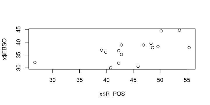<!-- --> --- ## R — ggplot Plotting with `ggplot2` - "grammar of graphics" - a plot is treated as a combination of various elements - minimal usage: provide `ggplot` with: - the data to use - aesthetics (how to map the variables in the data to visual properties of the plot) - geometries (what to show on the plot: points, lines, etc) --- ## R — ggplot ```r library(ggplot2) ggplot(x, aes(x = R_POS, y = FBSO)) + geom_point() ``` 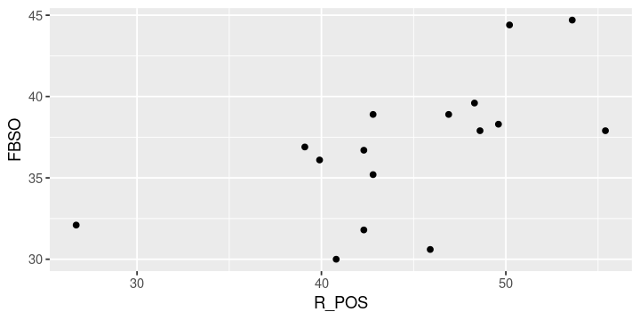<!-- --> --- ## R — ggplot ```r ggplot(x, aes(x = R_POS, y = FBSO)) + geom_point(`aes(col = Team)`) ``` 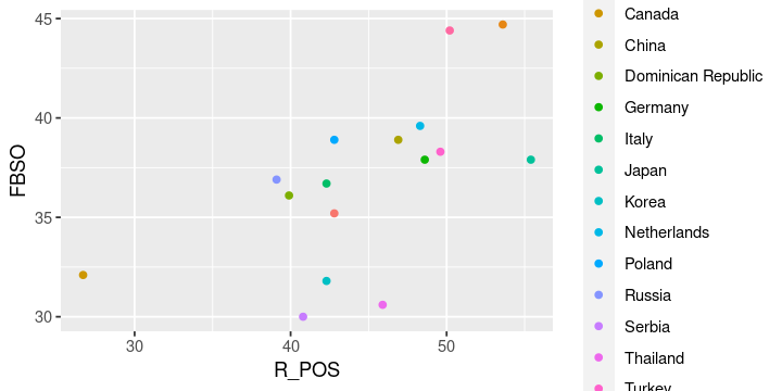<!-- --> --- ## R — ggplot ```r ggplot(x, aes(x = R_POS, y = FBSO)) + geom_point(`col = "red"`) + `geom_text(aes(label = Team))` ``` 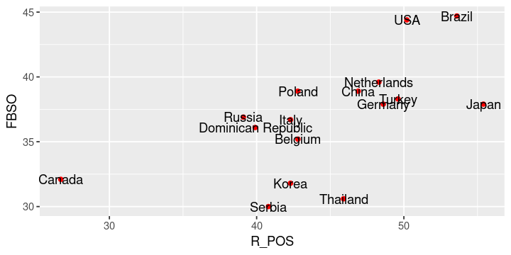<!-- --> --- ## R — ggplot ```r ggplot(x, aes(x = R_POS, y = FBSO)) + geom_point(col = "red") + geom_text(aes(label = Team)`, hjust = -0.1`) ``` <!-- --> --- ## R — ggplot ```r ggplot(x, aes(x = R_POS, y = FBSO)) + geom_point(col = "red") + geom_text(aes(label = Team), hjust = -0.1)` + xlim(c(NA, 58))` ``` <!-- --> --- ## R — ggplot ```r ggplot(x, aes(x = R_POS, y = FBSO)) + geom_point(col = "red") + `geom_smooth(method = "lm", se = FALSE) +` geom_text(aes(label = Team), hjust = -0.1) + xlim(c(NA, 58)) ``` <!-- --> --- ## R — ggplot ```r ggplot(x, aes(x = R_POS, y = FBSO)) + geom_point(col = "red") + geom_smooth(method = "lm", se = FALSE) + `theme_bw() +` geom_text(aes(label = Team), hjust = -0.1) + xlim(c(NA, 58)) + `labs(x = "Positive/perfect reception %", y = "First ball sideout %")` ``` <!-- --> --- ## R — ggplot: other geometries ```r ggplot(x, aes(x = REC_ATT_EFF)) + `geom_histogram`(binwidth = 2.5, col = "black", fill = "grey50") + theme_bw() + labs(x = "Reception attack efficiency") ``` 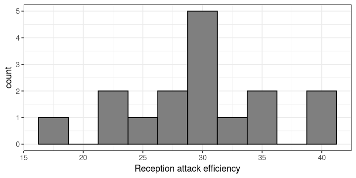<!-- --> --- ## R — ggplot: subplots (facets) ```r ggplot(x, aes(x = REC_ATT_EFF)) + geom_histogram(binwidth = 2.5, col = "black", fill = "grey50") + `facet_wrap(~Status)` + theme_bw() + labs(x = "Reception attack efficiency") ``` 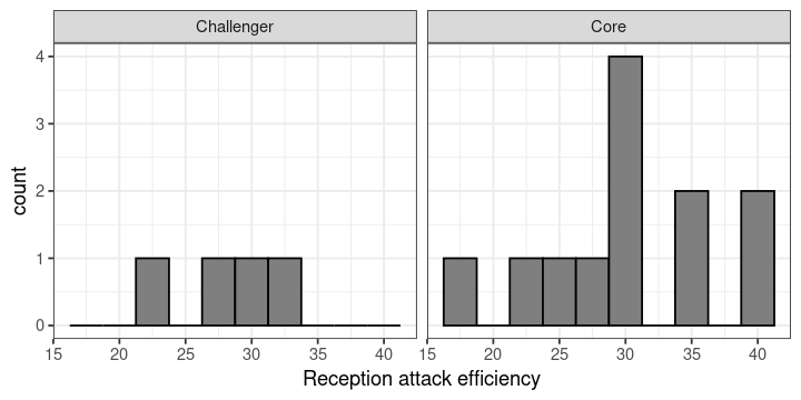<!-- --> --- ## R — Getting help - on specific functions or packages - `? function_name`, equivalently `help("function_name")` - package vignettes - general R - the [R-help mailing list](https://stat.ethz.ch/mailman/listinfo/r-help), [stackoverflow.com](https://stackoverflow.com) - volleyball-specific - the openvolley Slack - https://openvolley.org/volley-analytics-snippets - found a bug? Have a suggestion? Raise an issue on GitHub --- ## R — Exercises Open `s1-exercises.Rmd` in Rstudio, or `s1-exercises.html` in a browser.