Installation
## install.packages("remotes")
remotes::install_github("openvolley/ovml")
The ovml package provides image and video machine learning tools for volleyball analytics. See also the opensportml for a generalized version of this package for use with other sports.
Currently three versions of the YOLO object detection algorithm are included (versions 3, 4, and 7). These have been implemented on top of the torch R package, meaning that no Python installation is required on your system.
The package also includes an experimental network specifically for detecting volleyballs.
This implementation drew from ayooshkathuria/pytorch-yolo-v3, walktree/libtorch-yolov3, rockyzhengwu/libtorch-yolov4, gwinndr/YOLOv4-Pytorch, and WongKinYiu/yolov7.
Example
Use a YOLOv4 network to recognize objects in an image. We use a video frame image (bundled with the package):
library(ovml)
img <- ovml_example_image()
ovml_ggplot(img)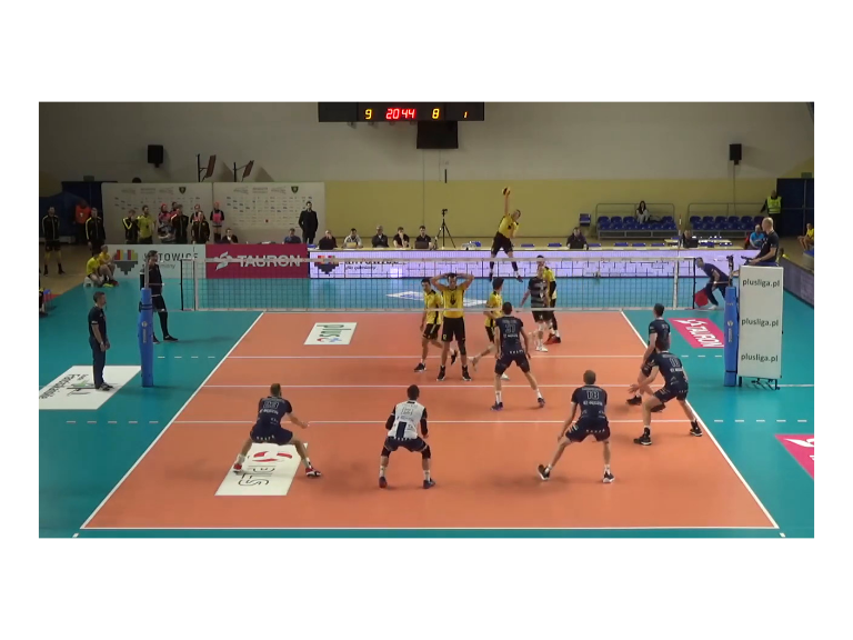
Construct the network. The first time this function is run, it will download and cache the network weights file (~250MB).
dn <- ovml_yolo()Now we can use the network to detect objects in our image:
dets <- ovml_yolo_detect(dn, img, conf = 0.3)
dets <- dets[dets$class %in% c("person", "sports ball"), ]
ovml_ggplot(img, dets)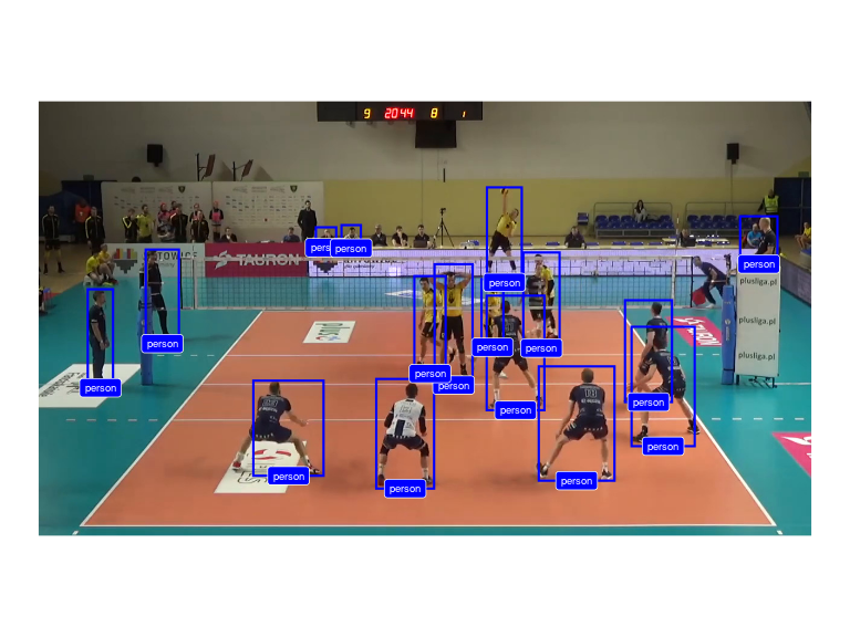
Note that this network didn’t detect the volleyball (in the process of being contacted by the server). Let’s try the experimental volleyball-specific network:
dn <- ovml_yolo("4-mvb")
ball_dets <- ovml_yolo_detect(dn, img)
ovml_ggplot(img, ball_dets, label_geom = NULL) ## don't add the label, it obscures the volleyball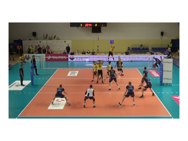
We can transform the image detections to real-world court coordinates. First we need to define the court reference points needed for the transformation. We can use the ov_shiny_court_ref helper app for this:
library(ovideo)
ref <- ov_shiny_court_ref(img)
ref should look something like:
ref
#> $antenna
#> # A tibble: 4 × 4
#>   image_x image_y antenna where
#>     <dbl>   <dbl> <chr>   <chr>
#> 1   0.208   0.348 left    floor
#> 2   0.82    0.353 right   floor
#> 3   0.823   0.641 right   net_top
#> 4   0.2     0.643 left    net_top
#>
#> $video_width
#> [1] 1280
#>
#> $video_height
#> [1] 720
#>
#> $video_framerate
#> [1] 30
#>
#> $net_height
#> [1] 2.43
#>
#> $court_ref
#> # A tibble: 4 × 4
#>   image_x image_y court_x court_y
#>     <dbl>   <dbl>   <dbl>   <dbl>
#> 1  0.0549  0.0221     0.5     0.5
#> 2  0.953   0.0233     3.5     0.5
#> 3  0.751   0.52       3.5     6.5
#> 4  0.289   0.516      0.5     6.5
Now use it with the ov_transform_points function (note that currently this function expects the image coordinates to be normalized with respect to the image width and height):
court_xy <- ovideo::ov_transform_points(x = (dets$xmin + dets$xmax) / 2 / ref$video_width,
                                        y = dets$ymin / ref$video_height,
                                        ref = ref$court_ref, direction = "to_court")
dets <- cbind(dets, court_xy)
And plot it:
library(datavolley)
library(ggplot2)
ggplot(dets, aes(x, y)) + ggcourt(labels = NULL, court_colour = "indoor") + geom_point()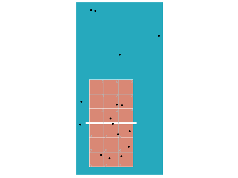
Keep in mind that ov_transform_points is using the middle-bottom of each bounding box and transforming it assuming that this represents a point on the court surface (the floor). Locations associated with truncated object boxes, or objects not on the court surface (players jumping, people in elevated positions such as the referee’s stand) will appear further away from the camera than they actually are.